9. 更多有用模块

本章节包含诸多快捷的模块方便配合EasyMultiProfiler数据分析流程使用。

9.1 多重字符串匹配检测 str_detect_multi

text <- c('Bacilli_unclassfiled','Bacteroidia_uncuture','Other')
str_detect_multi(text,c('Bacilli','bacteroidia'),exact=FALSE) # Ignore the capital letter
str_detect_multi(text,c('Bacilli','Bacteroidia'),exact=TRUE) # Set the matched completely

此外，在EasyMultiProfiler数据分析流程中，模块str_detect_multi也可以提供帮助。

🏷️示例1：可以同时提取微生物组学中门级别中Bacteroidetes和Firmicutes的物种。

MAE |> 
  EMP_assay_extract('taxonomy') |>
  EMP_filter(feature_condition = str_detect_multi(Phylum,c('Bacteroidetes','Firmicutes')))

🏷️示例2：可以剔除在纲级别没有完整注释的物种。

MAE |> 
  EMP_assay_extract('taxonomy') |>
  EMP_filter(feature_condition = !str_detect_multi(Class,'unclassified'))

9.2 兼容EasyMicroPlot数据分析流程 EMP_to_EMP1

在EasyMultiProfiler数据分析流程中，可以利用函数将微生物数据快速导出成EasyMicroPlot可接受的格式。

🏷️示例：导出微生物数据，并完成EasyMicroPlot的共发生网络分析。

# Get the data from EasyMultiProfiler
MAE |>
  EMP_assay_extract('taxonomy') |>
  EMP_feature_convert(from = 'tax_single',add = 'tax_full') |>
  EMP_to_EMP1(estimate_group = 'Group') -> deposit

# Work in the EasyMicroPlot
library(EasyMicroPlot)
cooc_re <- cooc_plot(data = deposit$data,design = deposit$mapping,
                     meta = deposit$meta,min_relative = 0.001,
                     min_ratio = 0.7,cooc_method'spearman',
                     cooc_output = TRUE)

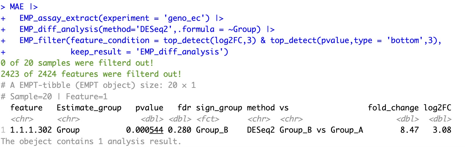
9.3 最大或者最小数值检测 top_detect

这个函数可以帮助EasyMultiProfiler数据分析流程快速筛选出想要的最高或者最低的数据。

🏷️示例： 选出差异分析中，log2FC最大的三个特征与pvalue最小的三个特征的交集。

MAE |>
  EMP_assay_extract(experiment = 'geno_ec') |>
  EMP_diff_analysis(method='DESeq2',.formula = ~Group) |>
  EMP_filter(feature_condition = top_detect(log2FC,3) & top_detect(pvalue,type = 'bottom',3) ,
             keep_result = 'EMP_diff_analysis')

9.4 多组差异分析 stat_test

此函数能够针对表格，快速实现多组件的差异分析比较，并自动设置合适的位置辅助ggplot2绘图。

🏷️示例1： 常规比较

data(ToothGrowth)

# 指定分组
stat_test(
  data = ToothGrowth,
  estimate_group = 'dose',
  value = 'len',
  method = "t.test"
) 
# 使用公式
stat_test(
  data = ToothGrowth,
  formula = len ~ dose,
  method = "t.test"
)

🏷️示例2： 亚组比较

data(ToothGrowth)

# 指定分组
stat_test(
  data = ToothGrowth,
  value = 'len',
  estimate_group = "supp",
  compare_group = "dose",
  method = "t.test"
)
# 使用公式
stat_test(
  data = ToothGrowth,
  estimate_group = 'supp',
  formula = len ~ dose,
  method = "t.test"
)

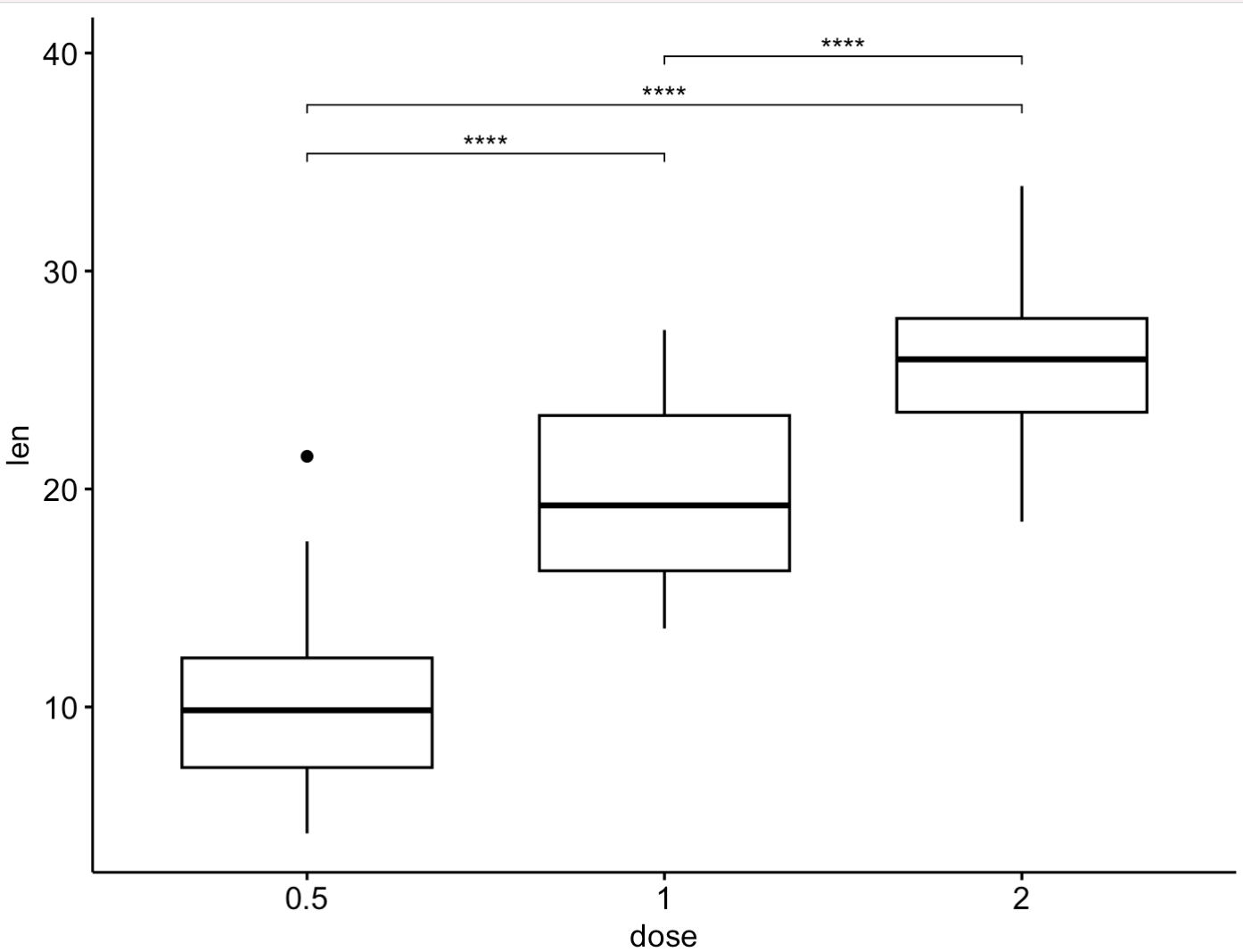
🏷️示例3： 对接ggplot2图形

stat_result <- stat_test(
  data = ToothGrowth,
  formula = len ~ dose,
  value = 'len',
  method = "tukey.hsd",
) 

# for ggpubr
if(require("ggpubr")){
  ggboxplot(ToothGrowth, x = "dose", y = "len") +
    stat_pvalue_manual(stat_result, label = "p.signif", tip.length = 0.01)
}